More Accurate ITS
Two model-agnostic solutions to enhance deep learning–based traffic forecasting.
This project explores model-agnostic approaches for enhancing the performance of deep learning–based traffic forecasting, which is composed of two publications:
- Error adjustment based on spatiotemporal correlation fusion for traffic forecasting Information Fusion.
- A universal framework of spatiotemporal bias block for long-term traffic forecasting IEEE Transactions on Intelligent Transportation Systems.
1. Autocorrelated Error Adjustment for Traffic Forecasting
Research gap
Mean squared error (MSE) estimation is frequently misapplied in the training of deep learning–based numerical forecasting models. Specifically,
-
Most existing studies treat forecasting tasks as regression problems and adopt standard regression training frameworks to optimize forecasting models.
-
Suppose each training example is denoted by a pair $\langle x, y \rangle$, where $x$ represents the input features and $y$ the corresponding target. The goal of regression is to learn a function $f$ that models the conditional distribution $p(y \mid x)$. A widely used approach is maximum likelihood estimation (MLE), which seeks to maximize the likelihood of the observed data under the model distribution. Assuming errors follows a Gaussian distribution with variance $\sigma^2$, the general form of the MLE loss function is:
- When the errors are assumed to be independent and identically distributed (i.i.d.), the variance term $\sigma^2$ becomes constant. In this case, maximizing the likelihood is equivalent to minimizing the mean squared error (MSE), which simplifies the training objective:
-
MSE is simple, computationally efficient, and widely used in practice. In standard regression tasks, where training samples are typically assumed to be randomly drawn from a distribution, the i.i.d. assumption holds reasonably well.
-
Existing time series forecasting studies adopt this same regression-based training paradigm, implicitly relying on the i.i.d. error assumption. However, Adjusting for Autocorrelated Errors in Neural Networks for Time Series (NeurIPS 2021) was among the first to question this assumption in univariate forecasting, showing that autocorrelated errors in the temporal dimension can negatively affect forecasting performance. Our work builds upon this insight and extends the discussion to the multivariate case, where spatial and temporal correlations in errors are even more prominent.
Solution
Model forecasting errors as a Vector Autoregressive (VAR) process instead of the i.i.d. assumption.
- Supposing $\epsilon_t$ represents the prediction error, traditional forecasting methods assume prediction errors are independent and identically distributed (i.i.d), typically $\epsilon_t \sim \mathcal{N}(\mathbf{0}, \Sigma)$. A one-step-ahead traffic forecasting model is typically formulated as:
-
The model is often trained by minimizing the loss functions $\text{MSE} \sim \sum\nolimits_t{|\epsilon_t|_2}$ and $\text{MAE} \sim \sum\nolimits_t{|\epsilon_t|_1}$, which correspond to independent Gaussian and independent Laplacian noise assumptions, respectively.
-
The independent noise assumption does not hold in real-world traffic forecasting, to account for spatiotemporal autocorrelation, we redefine the error term $\epsilon_t$ as $\eta_t$:
- In Eq.(1-4), $\epsilon_{t} \sim N(\boldsymbol{0},\Sigma)$ is a Gaussian white noise process, and $\Phi_{1},…,\Phi_{p}$ are coefficient matrices of size $N\times N$. We define $\eta_t$ to follow a vector autoregressive process VAR($p$):
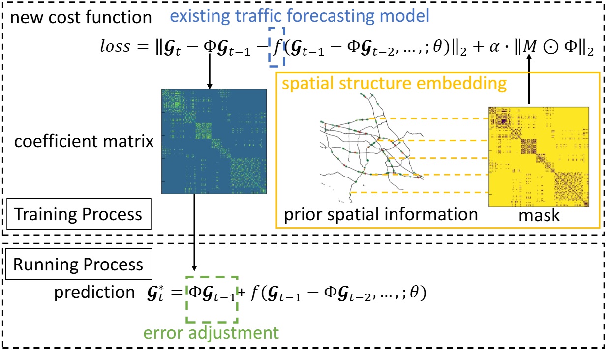
Redesign the loss function that explicitly incorporates spatiotemporal correlations.
- To adjust for autocorrelated errors, we employ a VAR(1) model in DNN-based traffic forecasting. By combining Eq.(1-4) and Eq.(1-5), the updated traffic forecasting model is formulated as:
- The historical prediction error, $\eta_{t-1}$, is computed as:
- Combining Eq.(1-6) and Eq.(1-7), we reformulate the traffic forecasting model as:
- This new formulation accounts for autocorrelated errors, but its complexity poses challenges in direct estimation. To simplify, we approximate the right-hand side of Eq.(1-8) as:
- Now, minimizing the independent Gaussian error, $\epsilon_t$, in Eq.(1-9), the final cost function used for training is updated as:
- Training with the new cost function, we can directly learn both the model parameter and the coefficient matrix.

2. Accumulated Error Adjustment for Long-Term Forecasting
Research gap
There are two general two approaches for multi-step traffic forecasting, namely: iterative multi-step forecasting and sequence-to-sequence (seq2seq) based forecasting. However, these two approaches have some major limitations, especially when it comes to long-term traffic forecasting (over 30 min in lead time).
-
The central idea of iterative multi-step scheme is to iteratively feed the output of current prediction as an input into the subsequent prediction.
-
However, the iterative use of previous results leads to accumulation of prediction errors throughout the whole process. Consequently, prediction errors of the said methods grow substantially with the length of prediction horizons.
-
The seq2seq-based models directly produce sequences of multi-period predictions.
-
Seq2seq models are typically computationally expensive to train, largely due to the convergence problems rooted in the high complexity of gradients computations when updating model parameters.
Solution
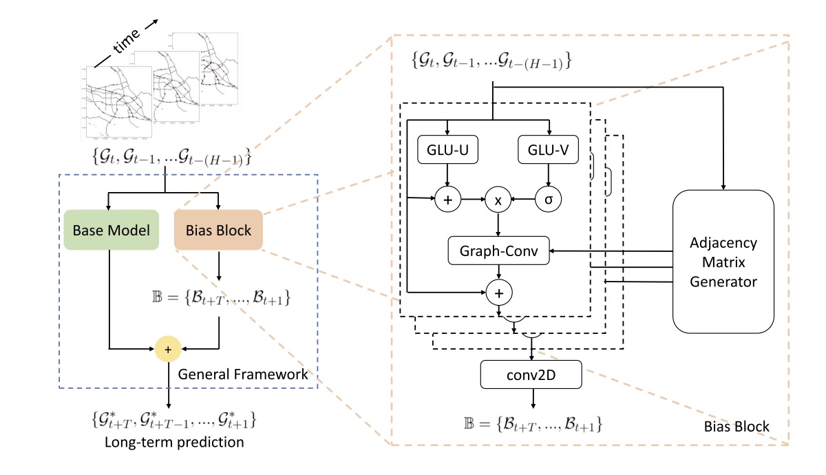
Overall structure of the uniform framework.
To enhance the long-term prediction ability of current forecasting models, we introduce the overall framework followed by the residual connection between the base model and bias block. The base model is a well-trained exsiting deep-learning-based forecasting methods, and the bias block is learnable to correct the long-term prediction error of the base model.

Supposing $f$ denotes the well-trained base model parameterized by $\Phi$ and $\mathbb{B}$ denotes the bias sequence, the universal framework integrates outputs of both the base model and bias block:
\[\{\mathcal{G}^{*}_{t+T},...\mathcal{G}^{*}_{t+1}\}= f(\{\mathcal{G}_{t},...\mathcal{G}_{t-(H-1)}\},\Phi)+\mathbb{B}. \tag{2-1}\]Supposing $f^{‘}$ denotes the bias block neural networks parameterized by $\Phi^{‘}$, the bias sequence, $\mathbb{B}$, is computed as:
\[\mathbb{B}=\{\mathcal{B}_{t+T},...,\mathcal{B}_{t+1}\}=f^{'}(\{\mathcal{G}_{t},...\mathcal{G}_{t-(H-1)}\},\Phi^{'}). \tag{2-2}\]Let $O_{base}$ denote the output of the base model and $L_{true}$ denote the ground truth in the training dataset. Parameters $\Phi$ of the base model are available since the base model is already well-trained. Thus, the framework only optimize $\Phi^{‘*}$—neural network parameters for the bias block:
\[\Phi^{'*}=\underset{\Phi^{'}}{\text{argmin}}\ O_{base}+f^{'}(\{\mathcal{G}_{t},...\mathcal{G}_{t-\left(H-1\right)}\},\Phi^{'})- L_{true}. \tag{2-3}\]Bias Block — Spatiotemporal Module.
The detailed structure of the bias block consists of three spatiotemporal modules, and an adjacency matrix generator used to provide the adjacency matrix to graph convolution operations. All three spatiotemporal modules share the same structure of a temporal layer and spatial layer. The temporal layer is composed of a dilated TCN with a gated mechanism. The output of the temporal layer is then fed into the spatial layer, which uses the graph convolution operation to capture the dynamic similarity between different vertices, and hidden/non-linear spatial patterns inside the traffic data.